A DEX Implied Volatility Proxy

Originally published on arXiv as A DEX Implied Volatility Proxy (arXiv:2608.13340, q-fin.MF, August 2026). This is a condensed summary. The full derivations, proofs, and empirical methodology are in the complete paper on arXiv.

The question

A narrow Uniswap v3 liquidity range behaves a lot like a short dated option: it earns fees while price stays inside the range and effectively expires the moment price crosses out of it. Panoptic builds on exactly this observation, streaming option premium through time as a function of price proximity and time in range rather than settling it upfront.

That resemblance motivates an obvious question: can something like implied volatility be extracted directly from Uniswap v3 and Panoptic using only on chain data, with no oracle at all?

A clean formula, and why it is too strong as written

Black-Scholes theta for a short dated option concentrates sharply around the strike as maturity goes to zero, mathematically converging to a scaled Dirac impulse. Matching that concentrated theta mass to the fee income earned by a narrow range LP position produces a strikingly simple closed form expression:

$$\sigma_{\text{fee}} = 2\, \text{feeRate}\sqrt{\frac{\text{Volume}}{L_{\text{tick}}}}$$

Every term on the right is a genuine on chain observable: the pool's fee tier, traded volume over a window, and active liquidity at the current tick. No price feed, no external volatility input.

The problem is what this formula actually captures. Fee income is only the compensation leg of a narrow range LP position. There is a second, unobserved leg: the cost of dynamically hedging the LP's negative convexity through arbitrage aligned trades that correct stale AMM prices after the market moves. That cost is formalized elsewhere in the AMM literature as predictable loss, or loss versus rebalancing (LVR), with an instantaneous rate of $\text{LVR} = \sigma^2/8$.

Fee income and hedging cost do not scale together. For a single price correcting move, fee income scales linearly with the size of the move, while the hedging cost scales quadratically, the AMM analogue of a convexity cost. Because those two legs move at different rates as volume changes, there is no fixed ratio between them, and matching theta to fees alone identifies only one side of the trade.

Why the structural volatility isn't identified

Formally: if fees only ever capture a fraction $\alpha$ of the true option cost, then $\sigma_{\text{fee}}^2 = \alpha\, \sigma_*^2$, where $\sigma_*$ is the structural volatility that would enter a genuine option pricing model. Unless $\alpha$ is known, every value of $\alpha \in (0, 1]$ implies a different $\sigma_*$ consistent with the exact same observed $\sigma_{\text{fee}}$. The mapping from pool data to a structural volatility is one to many.

Worse, $\alpha$ is not itself a simple pool state variable. It depends on the external efficient price process, the speed of arbitrage correction, the mix of informed versus uninformed flow, and the sampling scale, none of which are recoverable from aggregate fee accounting alone.

What the pool data support directly, then, is a fee implied activity index, not a Black-Scholes consistent implied volatility.

What the data actually show

Testing $\sigma_{\text{fee}}$ against realized volatility of ETH spot on the ETH/USDC 30bps pool, daily from January 2023 to July 2026, shows two things clearly.

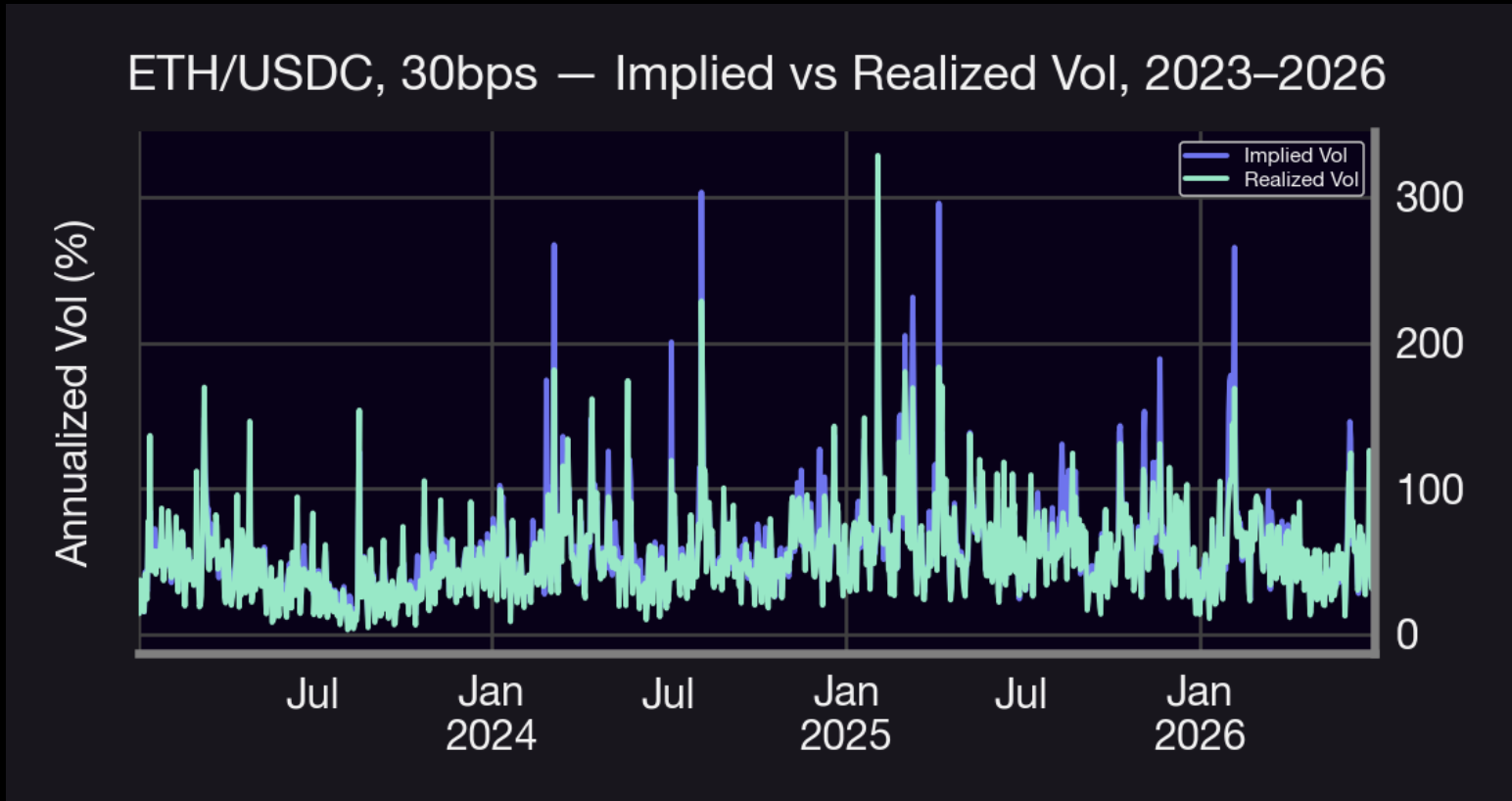
First, the fee implied proxy tracks realized volatility closely, a 0.87 correlation moving through the same compression and expansion regimes despite being built from entirely disjoint observables. That is exactly what you would want from a genuine activity index, even one that is not a structural volatility.

Second, the proxy consistently trades above realized volatility: a mean spread of 3.5 percentage points, above realized vol on 68% of days, with an implied capture ratio averaging 1.33.

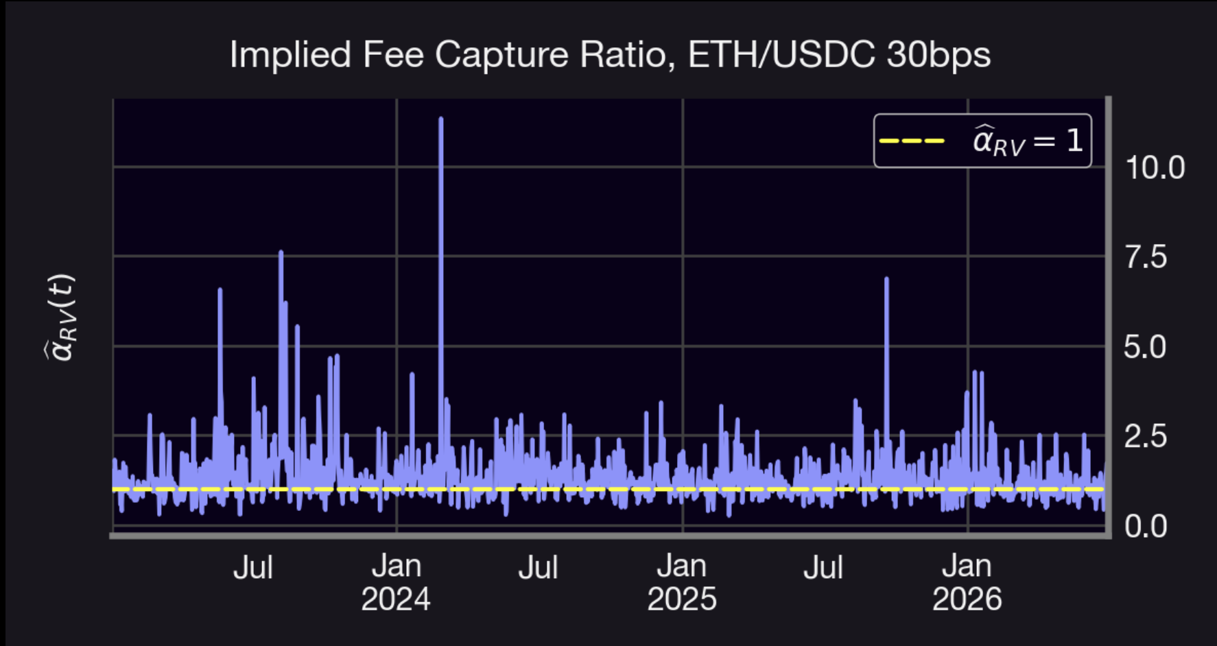
That premium is consistent with the volatility risk premium well documented in centralized options markets, where implied volatility trades above subsequently realized volatility because sellers price in compensation for bearing risk, not just its backward looking cost. But the paper is careful not to overclaim here: because the fee driven proxy can respond within the same window that generates it while realized volatility is backward looking by construction, part of this same pattern is a mechanical artifact of that lag, not necessarily a risk premium on its own.

Where this is useful, and where it is not

As an oracle free activity index, $\sigma_{\text{fee}}$ is well suited to scaling premium accrual schedules, comparing relative fee intensity across pools, informing collateral or margin buffers, and flagging unusual activity bursts relative to available liquidity.

It should not be read as a drop in replacement for a centralized exchange style implied volatility surface. Recovering that would require independently estimating the fee capture ratio $\alpha$, which needs a real microstructure filter separating arbitrage flow from uninformed flow, not just pool level fee and volume data.

Read the full paper

The complete paper includes the full Dirac delta derivation and proof, the tick spacing and fee tier mechanics underlying the matching convention, the non identification proposition in full, and the complete empirical methodology and summary statistics.

A DEX Implied Volatility Proxy — arXiv:2608.13340